
Contents
- Introduction
- Association Rule Mining
- Association Rule Mining on Titanic Data
- Algorithm Evaluation
- References
Introduction
In real world, We deal with various types of data for example date, currency, stock rate, categories and rank. These are all not same data types and also not easy to associate these all in single line information. There are lot of methods in Data Mining to extract the association or information from the complex data. Some methods are,
- Classification
- Estimation
- Prediction
- Affinity Grouping or Association Rules
- Clustering
- Anomaly Detection
In this post, I tried to explain the data mining process on Nominal Data Set.
The technique to extract the interesting information from Nominal data or Categorical data
is Association Rule Mining.
—
Association Rules Mining
Algorithms:
- Apriori
- FP Growth
Parameters:
- Support
- Ratio of the particular Object observation count to the total count.
- In another words, the percentage of a object strength in total strength.
- Range [0 - 1]
- Confidence
- How much confident association has with its pair.
- Range [0 - 1]
- Lift
- How much likely associated than individually occurred.
- Range [0 - inf]
- if lift > 1 means, It is an interesting scenario to consider.
- Leverage
- Range [-1, 1]
- If leverage =0 means, Both are independent.
- Conviction
- It is the metric to find the dependency on premise by the consequent.
- Range [0 - inf]
- If conviction = 1, items are independent.
- High Confident with Lower support. That means it is mostly depends on the another product.
Association Rule Mining on Titanic Data
Ready Up
Import Packages
import matplotlib.pyplot as plt
import pandas as pd
from mlxtend.preprocessing import TransactionEncoder
from mlxtend.frequent_patterns import apriori, association_rules

import warnings
warnings.filterwarnings("ignore")
import seaborn as sns
Loading Data-set
titanic = pd.read_csv('train.csv')
nominal_cols = ['Embarked','Pclass','Age', 'Survived', 'Sex']
cat_cols = ['Embarked','Pclass','Age', 'Survived', 'Title']
titanic['Title'] = titanic.Name.str.extract('\, ([A-Z][^ ]*\.)',expand=False)
titanic['Title'].fillna('Title_UK', inplace=True)
titanic['Embarked'].fillna('Unknown',inplace=True)
titanic['Age'].fillna(0, inplace=True)
# Replacing Binary with String
rep = {0: "Dead", 1: "Survived"}
titanic.replace({'Survived' : rep}, inplace=True)
Binning Age Column
## Binning Method to categorize the Continous Variables
def binning(col, cut_points, labels=None):
  minval = col.min()
  maxval = col.max()
  break_points = [minval] + cut_points + [maxval]
  if not labels:
    labels = range(len(cut_points)+1)
  colBin = pd.cut(col,bins=break_points,labels=labels,include_lowest=True)
  return colBin

cut_points = [1, 10, 20, 50 ]
labels = ["Unknown", "Child", "Teen", "Adult", "Old"]
titanic['Age'] = binning(titanic['Age'], cut_points, labels)
in_titanic = titanic[nominal_cols]
cat_titanic = titanic[cat_cols]
The data type of the Age column is converted from Number to Categorical using the method Binning. The data Set of the age column is ["Unknown", "Child", "Teen", "Adult", "Old"] and also ensured that all the columns are only have nominal data. The data set is separated into two types. They are,
- Gender Data
- Title Data
Gender Data
in_titanic.head()
| Embarked | Pclass | Age | Survived | Sex | |
|---|---|---|---|---|---|
| 0 | S | 3 | Adult | Dead | male |
| 1 | C | 1 | Adult | Survived | female |
| 2 | S | 3 | Adult | Survived | female |
| 3 | S | 1 | Adult | Survived | female |
| 4 | S | 3 | Adult | Dead | male |
Title Data
cat_titanic.head()
| Embarked | Pclass | Age | Survived | Title | |
|---|---|---|---|---|---|
| 0 | S | 3 | Adult | Dead | Mr. |
| 1 | C | 1 | Adult | Survived | Mrs. |
| 2 | S | 3 | Adult | Survived | Miss. |
| 3 | S | 1 | Adult | Survived | Mrs. |
| 4 | S | 3 | Adult | Dead | Mr. |
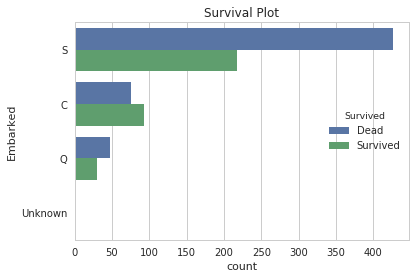
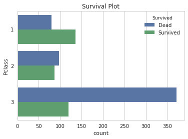
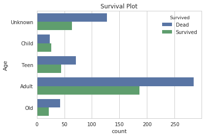
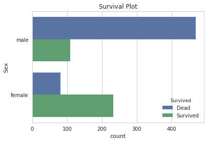
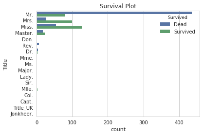
Data Visualization with Plots
for x in ['Embarked', 'Pclass','Age', 'Sex', 'Title']:
    sns.set(style="whitegrid")
    ax = sns.countplot(y=x, hue="Survived", data=titanic)
    plt.ylabel(x)
    plt.title('Survival Plot')
    plt.show()
Analysis - Methodology
- Gender Wise
- Title Wise
Because title is also a keyword which shows the Gender type of a person. Analysing these both fields together will cause for the results with 100% association with both fields.
Example:
- (Mr.) always associated with Male.
- (Mrs.) always associated with Female.
Putting these two fields together does not make any sense. So that the analysis split into two types.
Gender Analysis
dataset = []
for i in range(0, in_titanic.shape[0]-1):
    dataset.append([str(in_titanic.values[i,j]) for j in range(0, in_titanic.shape[1])])
# dataset = in_titanic.to_xarray()

oht = TransactionEncoder()
oht_ary = oht.fit(dataset).transform(dataset)
df = pd.DataFrame(oht_ary, columns=oht.columns_)
print df.head()
Output:
All Nominal Values
print oht.columns_
Output:
[‘1’, ‘2’, ‘3’, ‘Adult’, ‘C’, ‘Child’, ‘Dead’, ‘Old’, ‘Q’, ‘S’, ‘Survived’, ‘Teen’, ‘Unknown’, ‘female’, ‘male’]
Implementing Apriori Algorithm:
output = apriori(df, min_support=0.2, use_colnames=oht.columns_)
print output.head()
idx support itemsets 0 0.242697 (1) 1 0.206742 (2) 2 0.550562 (3) 3 0.528090 (Adult) 4 0.615730 (Dead)
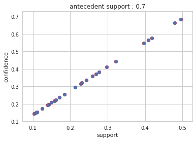
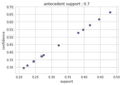
Rules Configuration
config = [
('antecedent support', 0.7),
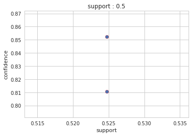
('support', 0.5),
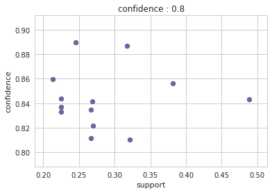
('confidence', 0.8),
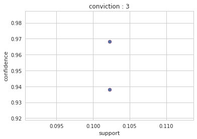
('conviction', 3)
]
for metric_type, th in config:
rules = association_rules(output, metric=metric_type, min_threshold=th)
if rules.empty:
print 'Empty Data Frame For Metric Type : ',metric_type,' on Threshold : ',th
continue
print rules.columns.values
print '-------------------------------------'
print 'Configuration : ', metric_type, ' : ', th
print '-------------------------------------'
print (rules)
support=rules.as_matrix(columns=['support'])
confidence=rules.as_matrix(columns=['confidence'])
plt.scatter(support, confidence, edgecolors='red')
plt.xlabel('support')
plt.ylabel('confidence')
plt.title(metric_type+' : '+str(th))
plt.show()
Output : Config 1: antecedent support = 0.7
Output : Config 2: antecedent support = 0.7
Output : Config 3: confidence: 0.8

Output : Config 4: conviction: 3
Gender Result
Interesting Information: Gender Analysis
- Persons Who are Sex: female With PcClass: 1, have 96.80 % Confidence Survived : True
- Persons Who are PcClass: 2 With Survived: False, have 93.81% Confidence Sex: Male
Common Information:
- Persons Who are Survived : False With Age : UnKnown , have 81.88 % Confidence PcClass : 3
- Persons Who are Age : Adult With PcClass : 2 , have 90.2 % Confidence Embarked : S
- Persons Who are Survived: False With Age : Adult and PcClass : 3, have 86.36% Confidence Embarked: S
Title Analysis
dataset = []
in_titanic=cat_titanic
for i in range(0, in_titanic.shape[0]-1):
    dataset.append([str(in_titanic.values[i,j]) for j in range(0, in_titanic.shape[1])])
# dataset = in_titanic.to_xarray()

oht = TransactionEncoder()
oht_ary = oht.fit(dataset).transform(dataset)
df = pd.DataFrame(oht_ary, columns=oht.columns_)
print df.head()
Output:
All Nominal values:
print oht.columns_
Output:
Implementing Apriori Algorithm:
output = apriori(df, min_support=0.2, use_colnames=oht.columns_)
print output.head()
support itemsets 0 0.242697 (1) 1 0.206742 (2) 2 0.550562 (3) 3 0.528090 (Adult) 4 0.615730 (Dead)
Rules Configuration
config = [
    ('antecedent support', 0.7),
    ('confidence', 0.8),
    ('conviction', 3)
]

for metric_type, th in config:
    rules = association_rules(output, metric=metric_type, min_threshold=th)
    if rules.empty:
        print 'Empty Data Frame For Metric Type : ',metric_type,' on Threshold : ',th
        continue
    print rules.columns.values
    print '-------------------------------------'
    print 'Configuration : ', metric_type, ' : ', th
    print '-------------------------------------'
    print (rules)

    support=rules.as_matrix(columns=['support'])
    confidence=rules.as_matrix(columns=['confidence'])

    plt.scatter(support, confidence, edgecolors='red')
    plt.xlabel('support')
    plt.ylabel('confidence')
    plt.title(metric_type+' : '+str(th))
    plt.show()
Output : Config 1: antecedent support = 0.7
Output : Config 2: confidence: 0.8
Output : Config 3: conviction: 3
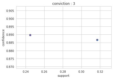
Title Result
Interesting Information - Title Analysis:
- Persons Who are Title : Mr. With Class : 3 and Embarked : S, have 88.9796 % Confidence Survived : Dead
How to filter ? - A simple Demo
rules[rules['confidence']==rules['confidence'].min()]
rules[rules['confidence']==rules['confidence'].max()]
Output Tables:
| antecedents | consequents | antecedent support | consequent support | support | confidence | lift | leverage | conviction | |
|---|---|---|---|---|---|---|---|---|---|
| 8 | (True) | (female) | 0.38427 | 0.352809 | 0.261798 | 0.681287 | 1.931035 | 0.126224 | 2.030636 |
| antecedents | consequents | antecedent support | consequent support | support | confidence | lift | leverage | conviction | |
|---|---|---|---|---|---|---|---|---|---|
| 12 | (1, female) | (True) | 0.105618 | 0.38427 | 0.102247 | 0.968085 | 2.519286 | 0.061661 | 19.292884 |
rules = association_rules (output, metric='support', min_threshold=0.1)
rules[rules['confidence'] == rules['confidence'].min()]
rules[rules['confidence'] == rules['confidence'].max()]
Output Tables:
| antecedents | consequents | antecedent support | consequent support | support | confidence | lift | leverage | conviction | |
|---|---|---|---|---|---|---|---|---|---|
| 274 | (S) | (True, Adult, female) | 0.723596 | 0.14382 | 0.103371 | 0.142857 | 0.993304 | -0.000697 | 0.998876 |
| antecedents | consequents | antecedent support | consequent support | support | confidence | lift | leverage | conviction | |
|---|---|---|---|---|---|---|---|---|---|
| 55 | (1, female) | (True) | 0.105618 | 0.38427 | 0.102247 | 0.968085 | 2.519286 | 0.061661 | 19.292884 |
Algorithm Evaluation
Use this Python script to evaluate the algorithms Apriori and FP Growth.
The evaluation output would be like,
Conclusion:
In terms of reading process, the algorithms Apriori and FP Growth differs. According to that FP Growth is more efficient than apriori for bigger data because it reads only two times a file. But for me both are working in same manner and almost consumes same time for a specific data. It may be differ with respect to the data and nominal value count. Any way before implementing these algorithm, once check with Algorithm-Evaluation</ark> as said before and find the suitable algorithm for your work.
Also published in Kaggle.
References:
Thanks to the Sources, - Apriori - FP Growth - Association Rule Mining Via Apriori Algorithm in python - Mining Frequent Items using apriori algorithm - Finding Frequent Patterns - Efficient - Apriori - Python 3.6 - Data mining with apriori
Related Posts
Design A Rectangular Patch Antenna Using Python
Learn Javascript Basics In 30 Minutes